Sharp regression discontinuity with pymc models

import causalpy as cp

%load_ext autoreload
%autoreload 2
%config InlineBackend.figure_format = 'retina'
seed = 42

df = cp.load_data("rd")

Linear, main-effects, and interaction model

Note

The random_seed keyword argument for the PyMC sampler is not necessary. We use it here so that the results are reproducible.

result = cp.RegressionDiscontinuity(
    df,
    formula="y ~ 1 + x + treated + x:treated",
    model=cp.pymc_models.LinearRegression(sample_kwargs={"random_seed": seed}),
    treatment_threshold=0.5,
)

fig, ax = result.plot()
fig

Initializing NUTS using jitter+adapt_diag...
Multiprocess sampling (4 chains in 4 jobs)
NUTS: [beta, y_hat_sigma]

Sampling 4 chains for 1_000 tune and 1_000 draw iterations (4_000 + 4_000 draws total) took 2 seconds.
Sampling: [beta, y_hat, y_hat_sigma]
Sampling: [y_hat]
Sampling: [y_hat]
Sampling: [y_hat]
Sampling: [y_hat]

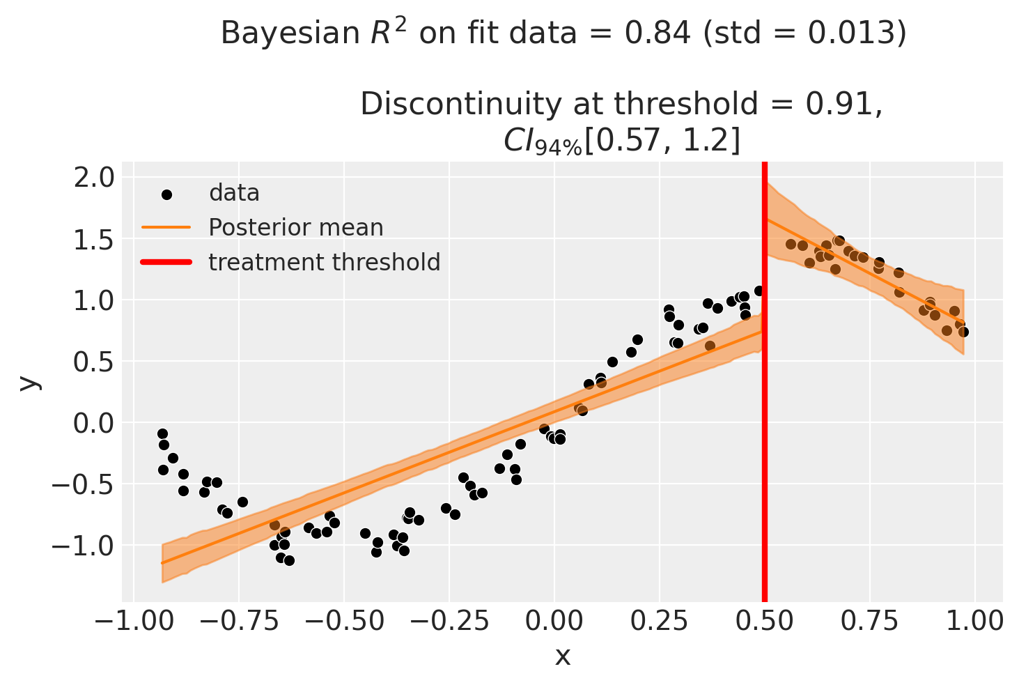
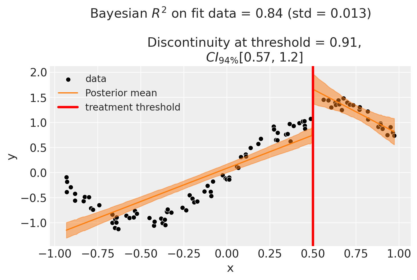
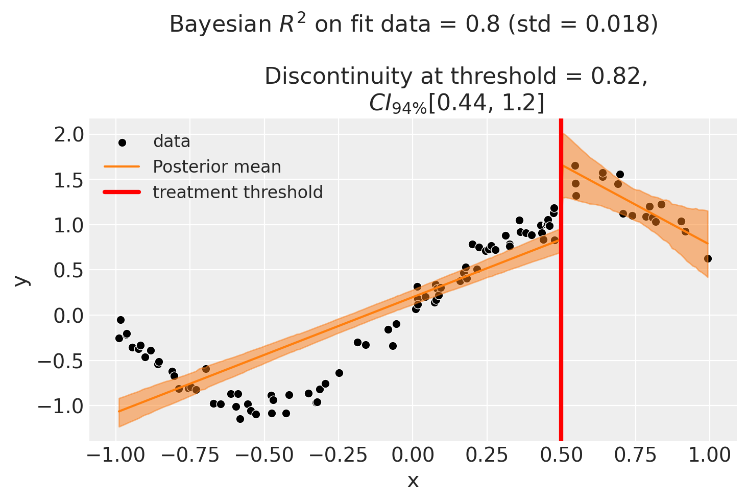
Though we can see that this does not give a good fit of the data almost certainly overestimates the discontinuity at threshold.

Using a bandwidth

One way how we could deal with this is to use the bandwidth kwarg. This will only fit the model to data within a certain bandwidth of the threshold. If \(x\) is the running variable, then the model will only be fitted to data where \(threshold - bandwidth \le x \le threshold + bandwidth\).

result = cp.RegressionDiscontinuity(
    df,
    formula="y ~ 1 + x + treated + x:treated",
    model=cp.pymc_models.LinearRegression(sample_kwargs={"random_seed": seed}),
    treatment_threshold=0.5,
    bandwidth=0.3,
)

fig, ax = result.plot()

Initializing NUTS using jitter+adapt_diag...
Multiprocess sampling (4 chains in 4 jobs)
NUTS: [beta, y_hat_sigma]

Sampling 4 chains for 1_000 tune and 1_000 draw iterations (4_000 + 4_000 draws total) took 3 seconds.
There was 1 divergence after tuning. Increase `target_accept` or reparameterize.
Sampling: [beta, y_hat, y_hat_sigma]
Sampling: [y_hat]
Sampling: [y_hat]
Sampling: [y_hat]
Sampling: [y_hat]

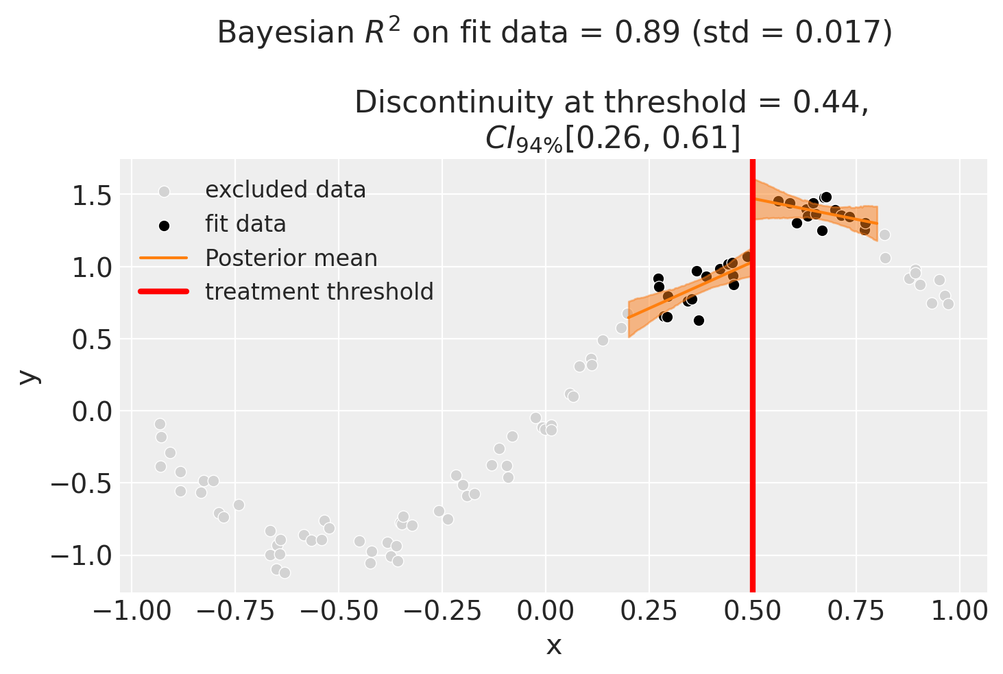
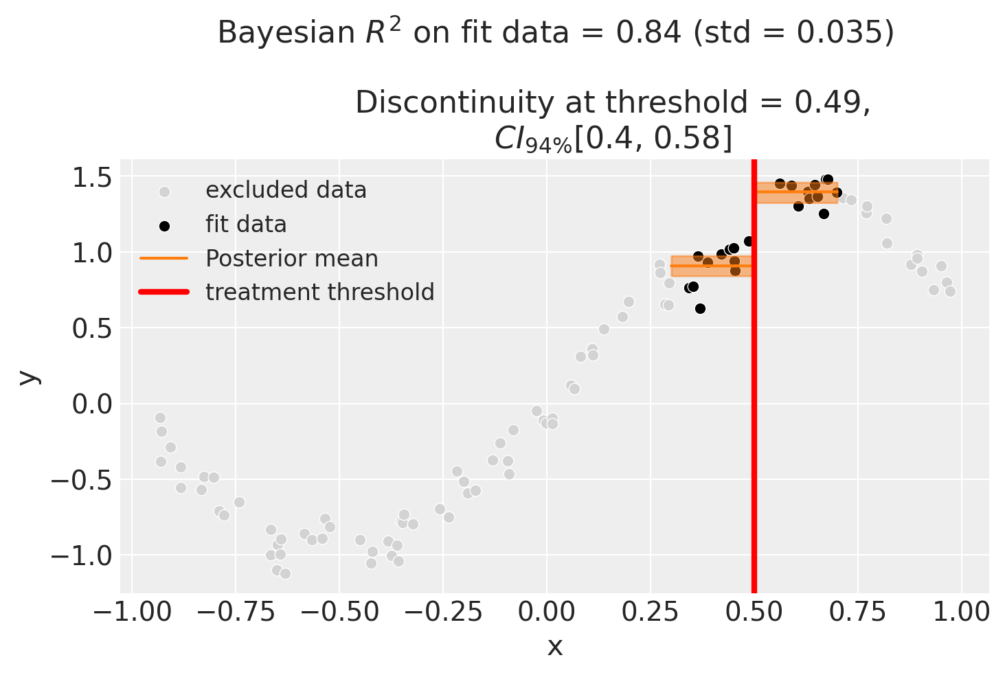
We could even go crazy and just fit intercepts for the data close to the threshold. But clearly this will involve more estimation error as we are using less data.

result = cp.RegressionDiscontinuity(
    df,
    formula="y ~ 1 + treated",
    model=cp.pymc_models.LinearRegression(sample_kwargs={"random_seed": seed}),
    treatment_threshold=0.5,
    bandwidth=0.2,
)

fig, ax = result.plot()

Initializing NUTS using jitter+adapt_diag...
Multiprocess sampling (4 chains in 4 jobs)
NUTS: [beta, y_hat_sigma]

Sampling 4 chains for 1_000 tune and 1_000 draw iterations (4_000 + 4_000 draws total) took 1 seconds.
Sampling: [beta, y_hat, y_hat_sigma]
Sampling: [y_hat]
Sampling: [y_hat]
Sampling: [y_hat]
Sampling: [y_hat]

Using basis splines

Though it could arguably be better to fit with a more complex model, fit example a spline. This allows us to use all of the data, and (depending on the situation) maybe give a better fit.

result = cp.RegressionDiscontinuity(
    df,
    formula="y ~ 1 + bs(x, df=6) + treated",
    model=cp.pymc_models.LinearRegression(sample_kwargs={"random_seed": seed}),
    treatment_threshold=0.5,
)

fig, ax = result.plot()

Initializing NUTS using jitter+adapt_diag...
Multiprocess sampling (4 chains in 4 jobs)
NUTS: [beta, y_hat_sigma]

Sampling 4 chains for 1_000 tune and 1_000 draw iterations (4_000 + 4_000 draws total) took 1 seconds.
Sampling: [beta, y_hat, y_hat_sigma]
Sampling: [y_hat]
Sampling: [y_hat]
Sampling: [y_hat]
Sampling: [y_hat]

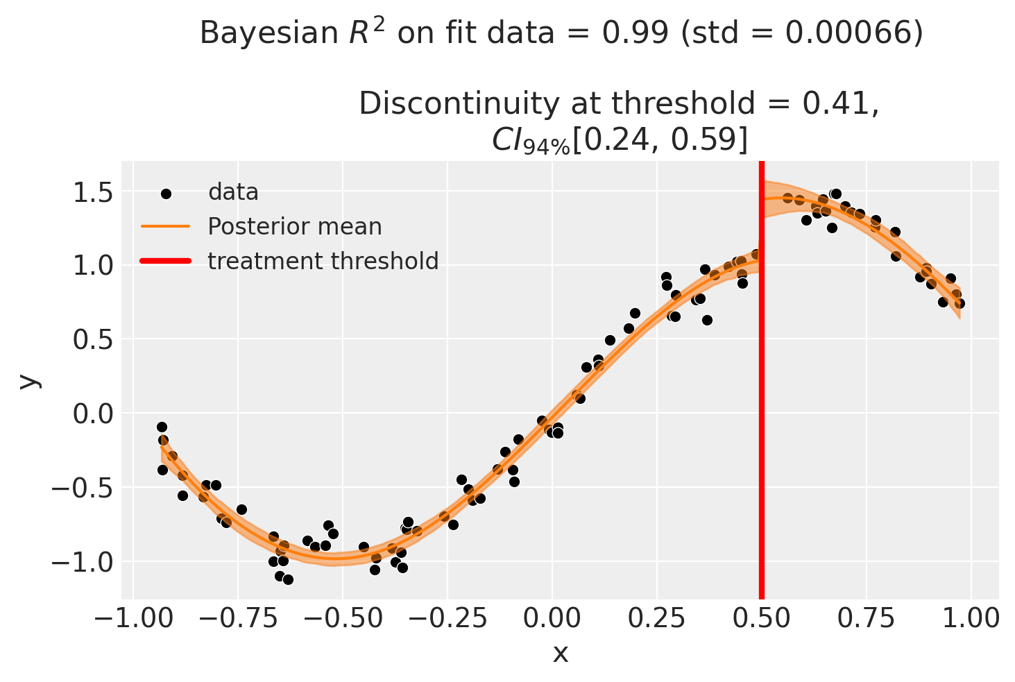
As with all of the models in this notebook, we can ask for a summary of the model coefficients.

result.summary()

Regression Discontinuity experiment
Formula: y ~ 1 + bs(x, df=6) + treated
Running variable: x
Threshold on running variable: 0.5
Bandwidth: inf
Donut hole: 0.0
Observations used for fit: 100

Results:
Discontinuity at threshold = 0.41$CI_{94\%}$[0.24, 0.59]


Model coefficients:
    Intercept        -0.23, 94% HDI [-0.32, -0.14]
    treated[T.True]  0.41, 94% HDI [0.24, 0.59]
    bs(x, df=6)[0]   -0.6, 94% HDI [-0.78, -0.41]
    bs(x, df=6)[1]   -1.1, 94% HDI [-1.2, -0.93]
    bs(x, df=6)[2]   0.28, 94% HDI [0.12, 0.43]
    bs(x, df=6)[3]   1.7, 94% HDI [1.5, 1.8]
    bs(x, df=6)[4]   1, 94% HDI [0.66, 1.4]
    bs(x, df=6)[5]   0.56, 94% HDI [0.36, 0.75]
    y_hat_sigma      0.1, 94% HDI [0.089, 0.12]

We can get nicely formatted tables from our integration with the maketables package.

from maketables import ETable

result.set_maketables_options(hdi_prob=0.95)
ETable(result, coef_fmt="b:.3f \n [ci95l:.3f, ci95u:.3f]")

	y
	(1)
coef
treated=True	0.410 [0.238, 0.602]
bs(x, df=6)=0	-0.596 [-0.784, -0.398]
bs(x, df=6)=1	-1.073 [-1.218, -0.930]
bs(x, df=6)=2	0.276 [0.111, 0.428]
bs(x, df=6)=3	1.652 [1.486, 1.810]
bs(x, df=6)=4	1.020 [0.653, 1.381]
bs(x, df=6)=5	0.562 [0.356, 0.751]
Intercept	-0.231 [-0.334, -0.141]
stats
N	100
Bayesian R2	0.986
Format of coefficient cell: Coefficient [95% CI Lower, 95% CI Upper]

Effect Summary Reporting

For decision-making, you often need a concise summary of the causal effect. The effect_summary() method provides a decision-ready report with key statistics. Note that for Regression Discontinuity, the effect is a single scalar (the discontinuity at the threshold), similar to Difference-in-Differences.

# Generate effect summary
stats = result.effect_summary()
stats.table

	mean	median	hdi_lower	hdi_upper	p_gt_0
discontinuity	0.411137	0.409325	0.239555	0.601715	1.0

print(stats.text)

The discontinuity at threshold was 0.41 (95% HDI [0.24, 0.60]), with a posterior probability of an increase of 1.000.

You can customize the summary with different directions and ROPE thresholds:

• Direction: Test for increase, decrease, or two-sided effect

• Alpha: Set the HDI confidence level (default 95%)

• ROPE: Specify a minimal effect size threshold

# Example: Two-sided test with ROPE
stats = result.effect_summary(
    direction="two-sided",
    alpha=0.05,
    min_effect=0.2,  # Region of Practical Equivalence
)
stats.table

	mean	median	hdi_lower	hdi_upper	p_two_sided	prob_of_effect	p_rope
discontinuity	0.411137	0.409325	0.239555	0.601715	0.0	1.0	0.99125

print("\n" + stats.text)

The discontinuity at threshold was 0.41 (95% HDI [0.24, 0.60]), with a posterior probability of an effect of 1.000.

Sensitivity analysis

This section walks through the Regression discontinuity design sensitivity diagnostics that ship with the pipeline API (EstimateEffect → SensitivityAnalysis → GenerateReport). For the shared workflow concepts—Pipeline, pluggable checks, and HTML reports—see Pipeline Workflow. For the matrix of which checks apply to which experiment type, see Sensitivity Checks in Pipeline Workflows.

Related checks

For sharp RD designs, the pipeline currently exposes the following checks:

• BandwidthSensitivity (below) — re-fits the experiment at a sequence of bandwidths and reports the estimated discontinuity at each. Targets the bias–variance trade-off in local designs [Imbens and Lemieux, 2008, Lee and Lemieux, 2010].

• McCraryDensityTest (below) — looks for a discontinuity in the density of the running variable at the threshold, which would indicate possible manipulation of assignment [McCrary, 2008].

• PriorSensitivity — re-fits the same specification with alternative PyMCModel priors. It complements bandwidth and density diagnostics but does not replace them.

PlaceboInTime, LeaveOneOut, and PlaceboInSpace target other estimator families (ITS, Synthetic Control) and are not applicable to a sharp RD fit.

Walkthrough

1. Fit a baseline model so you have a reference effect estimate (the linear interaction model fitted at the top of this notebook plays that role).

2. Run the pipeline cell below. It refits the experiment using cp.RegressionDiscontinuity inside EstimateEffect, then runs both BandwidthSensitivity and McCraryDensityTest. Each CheckResult exposes text (human-readable verdict), an optional table (per-bandwidth estimates or density counts), and metadata.

3. Inspect the per-check tables to compare the discontinuity estimate across bandwidths and to read off the McCrary z-statistic and p-value.

4. Open the HTML report (iframe) for a consolidated view alongside the main estimate.

Note

The bandwidth sweep below uses the linear interaction model y ~ 1 + x + treated + x:treated rather than the basis-spline specification. This is intentional: when basis splines like bs(x, df=6) are fit on the full data, the knot positions are baked in and patsy raises an error if a narrower bandwidth subset asks the model to evaluate observations that are inside the bandwidth window but where some training rows would now sit outside the original outer knots. The linear interaction formula has no such constraint and is the most common reference specification for bandwidth sensitivity studies in any case.

sensitivity_result = cp.Pipeline(
    data=df,
    steps=[
        cp.EstimateEffect(
            method=cp.RegressionDiscontinuity,
            formula="y ~ 1 + x + treated + x:treated",
            model=cp.pymc_models.LinearRegression(sample_kwargs={"random_seed": seed}),
            treatment_threshold=0.5,
        ),
        cp.SensitivityAnalysis(
            checks=[
                cp.checks.BandwidthSensitivity(bandwidths=[0.1, 0.2, 0.3, 0.5, 1.0]),
                cp.checks.McCraryDensityTest(n_bins=20),
            ],
        ),
        cp.GenerateReport(include_plots=True),
    ],
).run()

for cr in sensitivity_result.sensitivity_results:
    print(f"[{cr.check_name}] {cr.text}")

Initializing NUTS using jitter+adapt_diag...

Multiprocess sampling (4 chains in 4 jobs)

NUTS: [beta, y_hat_sigma]

Sampling 4 chains for 1_000 tune and 1_000 draw iterations (4_000 + 4_000 draws total) took 2 seconds.

Sampling: [beta, y_hat, y_hat_sigma]

Sampling: [y_hat]

Sampling: [y_hat]

Sampling: [y_hat]

Sampling: [y_hat]

Initializing NUTS using jitter+adapt_diag...

Multiprocess sampling (4 chains in 4 jobs)

NUTS: [beta, y_hat_sigma]

Sampling 4 chains for 1_000 tune and 1_000 draw iterations (4_000 + 4_000 draws total) took 33 seconds.

There were 239 divergences after tuning. Increase `target_accept` or reparameterize.

Chain 1 reached the maximum tree depth. Increase `max_treedepth`, increase `target_accept` or reparameterize.

Chain 2 reached the maximum tree depth. Increase `max_treedepth`, increase `target_accept` or reparameterize.

Sampling: [beta, y_hat, y_hat_sigma]

Sampling: [y_hat]

Sampling: [y_hat]

Sampling: [y_hat]

Sampling: [y_hat]

Initializing NUTS using jitter+adapt_diag...

Multiprocess sampling (4 chains in 4 jobs)

NUTS: [beta, y_hat_sigma]

Sampling 4 chains for 1_000 tune and 1_000 draw iterations (4_000 + 4_000 draws total) took 3 seconds.

There were 3 divergences after tuning. Increase `target_accept` or reparameterize.

Sampling: [beta, y_hat, y_hat_sigma]

Sampling: [y_hat]

Sampling: [y_hat]

Sampling: [y_hat]

Sampling: [y_hat]

Initializing NUTS using jitter+adapt_diag...

Multiprocess sampling (4 chains in 4 jobs)

NUTS: [beta, y_hat_sigma]

Sampling 4 chains for 1_000 tune and 1_000 draw iterations (4_000 + 4_000 draws total) took 2 seconds.

Sampling: [beta, y_hat, y_hat_sigma]

Sampling: [y_hat]

Sampling: [y_hat]

Sampling: [y_hat]

Sampling: [y_hat]

Initializing NUTS using jitter+adapt_diag...

Multiprocess sampling (4 chains in 4 jobs)

NUTS: [beta, y_hat_sigma]

Sampling 4 chains for 1_000 tune and 1_000 draw iterations (4_000 + 4_000 draws total) took 2 seconds.

Sampling: [beta, y_hat, y_hat_sigma]

Sampling: [y_hat]

Sampling: [y_hat]

Sampling: [y_hat]

Sampling: [y_hat]

Initializing NUTS using jitter+adapt_diag...

Multiprocess sampling (4 chains in 4 jobs)

NUTS: [beta, y_hat_sigma]

Sampling 4 chains for 1_000 tune and 1_000 draw iterations (4_000 + 4_000 draws total) took 2 seconds.

Sampling: [beta, y_hat, y_hat_sigma]

Sampling: [y_hat]

Sampling: [y_hat]

Sampling: [y_hat]

Sampling: [y_hat]

[BandwidthSensitivity] Bandwidth sensitivity analysis: compared 5 bandwidth values. Examine the table for consistency of effect estimates across bandwidths.
[McCraryDensityTest] McCrary density test: possible manipulation detected at threshold 0.5 (z=8.785, p=0.000). Observations below: 83, above: 17.

import html as html_module
import warnings

from IPython.display import HTML

with warnings.catch_warnings():
    warnings.filterwarnings(
        "ignore", "Consider using IPython.display.IFrame", UserWarning
    )
    display(
        HTML(
            f'<iframe srcdoc="{html_module.escape(sensitivity_result.report)}" '
            f'width="100%" height="600" style="border:1px solid #ccc;"></iframe>'
        )
    )

Interpreting pass and fail

BandwidthSensitivity is informational (passed=None): it returns a table of estimates rather than a binary verdict. Read the column of effect estimates and HDIs across bandwidths and ask:

• Are the point estimates broadly consistent in sign and magnitude across plausible bandwidths?

• Do the HDIs overlap substantially?

• Does the estimate flip or change order of magnitude at extreme bandwidths only, or also at moderate ones?

A result that is stable across moderate bandwidths is more credible than one that depends on a single narrow window.

McCraryDensityTest returns a binary verdict. It passes when the proportion of observations on each side of the threshold is consistent with no discontinuity at the conventional significance level (default alpha=0.05). It fails when the proportions differ enough to suggest sorting around the threshold. In either case, treat the verdict as a screening signal rather than a definitive answer; the test in CausalPy is histogram-based and does not implement the local-polynomial density estimator from [McCrary, 2008] exactly.

Important

On the built-in rd dataset the McCrary check fails simply because the running variable is generated on [-1, 1] while the threshold sits at 0.5. The histogram-based test reads the resulting global imbalance as a discontinuity even though no manipulation occurred. Real diagnostics should be paired with knowledge of the data-generating process: if you know assignment is exogenous, a McCrary failure may reflect asymmetric ranges of the running variable rather than sorting. When manipulation is plausible, follow up with a donut RD design.

If these checks fail

Concrete steps when one or both checks raise concerns:

1. Bandwidth dependence. If the estimate changes sign or magnitude across bandwidths, plot the running variable and outcome together and look for non-linear structure away from the threshold that the model is absorbing. Try a richer functional form (basis splines, see Using basis splines above) or restrict to a more local bandwidth and report both.

2. Sparse data near the threshold. A narrow bandwidth with very few observations gives noisy estimates regardless of design quality. The BandwidthSensitivity rows surface this directly via missing or very wide HDIs. Consider whether the design supports a wider effective window.

3. Density discontinuity. A failed McCraryDensityTest suggests possible manipulation of the running variable. Investigate the data-generating process: are units close to the threshold able to influence their own assignment? When manipulation is plausible, a donut RD design that excludes observations immediately around the threshold is a standard robustness response.

4. Compare under alternative priors with PriorSensitivity. If both diagnostics raise concerns, re-fitting under tighter or more diffuse priors helps separate prior-data conflict from genuine design weakness.

See also

• Sensitivity Checks in Pipeline Workflows — full check matrix and interpretation guidance

• Pipeline Workflow — end-to-end pipeline tutorial

• HTML Report Generation — HTML report generation

• Donut Regression Discontinuity — donut RDD as a robustness response to suspected manipulation